The perceptron is one of the earliest and most elegant ideas in artificial neural networks. Introduced by Frank Rosenblatt in 1958 (and implemented on the Mark I Perceptron computer), it is essentially a single artificial neuron that makes a binary decision: yes/no, 0/1, fire/don’t fire. Despite its simplicity, the perceptron revealed something profound: networks of these basic units can — in theory — compute anything a digital computer can compute.
Let’s break it down step by step, exactly as described in the transcript.
1. How a Single Perceptron Works
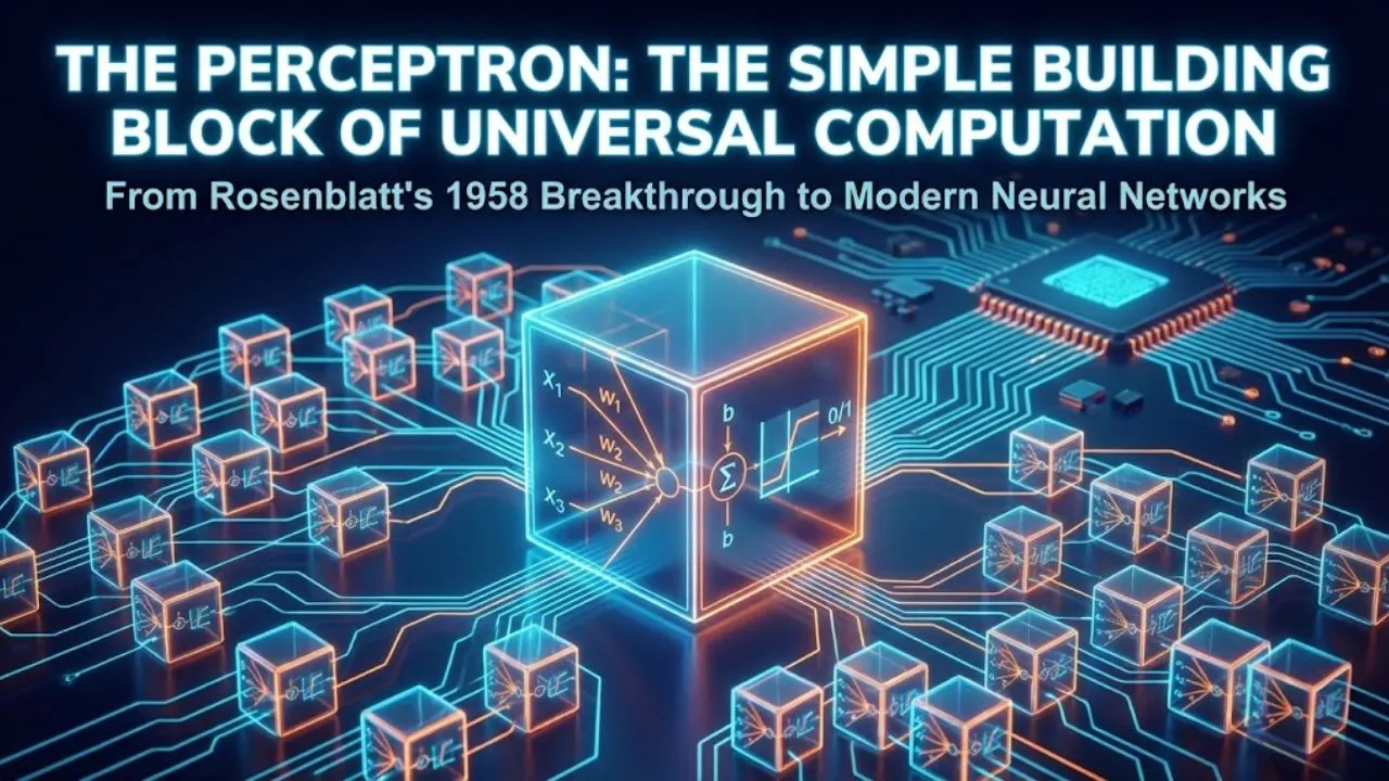
A perceptron takes several real-valued inputs (x₁, x₂, …, xₙ) and produces a single binary output (0 or 1).
Core computation:
- Each input xⱼ is multiplied by a corresponding weight wⱼ.
- All weighted inputs are summed → z = w₁x₁ + w₂x₂ + … + wₙxₙ + b (b is the bias — a constant that shifts the decision boundary)
- A simple activation function (also called the step function or Heaviside function) is applied to z:f(z) = { 1 if z > 0 { 0 if z ≤ 0
That’s it. No fancy non-linearities, no sigmoid, no ReLU — just a hard threshold.
In vector form: z = w · x + b output = 1 if z > 0 else 0
2. Real-World Intuition: “Should I Go to the Movies?”
Imagine deciding whether to go to the movies based on three binary factors (0 = no/bad, 1 = yes/good):
- x₁ = Weather is good
- x₂ = Have company
- x₃ = Theater is close (proximity)
Weights might be chosen like this (reflecting importance):
- w₁ = 4 (weather matters most)
- w₂ = 2
- w₃ = 2
- bias b = –5
Decision rule: Go (1) only if weather is good and at least one of company or proximity is true.
Examples:
- Bad weather (x₁=0), company yes (x₂=1), close yes (x₃=1) z = 0·4 + 1·2 + 1·2 – 5 = 4 – 5 = –1 ≤ 0 → Output = 0 (stay home)
- Good weather (x₁=1), company yes (x₂=1), close no (x₃=0) z = 1·4 + 1·2 + 0·2 – 5 = 6 – 5 = 1 > 0 → Output = 1 (go to movies)
The weights and bias create a linear decision boundary in input space.
3. Geometrically: A Linear Classifier
For two inputs (x₁, x₂), the equation w₁x₁ + w₂x₂ + b = 0 describes a straight line in 2D space.
Everything on one side of the line gives output 1, everything on the other side gives 0.
Example from transcript:
- w₁ = –2, w₂ = –2, b = 3
- Decision boundary: –2x₁ – 2x₂ + 3 = 0 → x₁ + x₂ = 1.5
- Left of line → z > 0 → output 1
- Right of line → z ≤ 0 → output 0
This is exactly what a linear binary classifier does — the same principle behind logistic regression, support vector machines (hard-margin case), and the decision boundaries in many early machine-learning models.
4. The Magic Discovery: Perceptrons Can Implement Logic Gates
Now assume inputs are strictly binary (0 or 1). A single perceptron can implement basic logic gates.
Most famously, a perceptron can act as a NAND gate (one of the most important gates in digital electronics):
| x₁ | x₂ | NAND (output) |
|---|---|---|
| 0 | 0 | 1 |
| 0 | 1 | 1 |
| 1 | 0 | 1 |
| 1 | 1 | 0 |
With weights w₁ = –2, w₂ = –2, bias b = 3, the perceptron exactly reproduces the NAND truth table.
Why is this huge? NAND is a universal logic gate. Every possible digital logic circuit (AND, OR, NOT, XOR, adders, multipliers, memory, CPUs…) can be built using only NAND gates.
Therefore: A network of perceptrons can implement any digital logic circuit → Perceptrons are computationally universal (in the boolean sense).
5. Example: Building a 1-Bit Adder with Perceptrons
A 1-bit adder takes two bits x₁, x₂ and produces:
- Sum bit = x₁ XOR x₂
- Carry bit = x₁ AND x₂
The standard NAND-gate implementation looks like this (text diagram approximation):
text
x₁ ─┬───── NAND ─┬───── NAND ──► Carry (x₁ AND x₂)
         │            │
         └───── NAND ─┘
               │
     x₂ ────────┘
               │
               └───── NAND ──► Sum (x₁ XOR x₂)
Since each NAND can be replaced by one perceptron (with appropriate weights & bias), the entire 1-bit adder becomes a small feedforward network of perceptrons.
This was a stunning insight in the late 1950s–early 1960s: simple threshold units arranged in layers could — in principle — compute anything.
Why the Perceptron Still Matters in 2026
Even though modern neural networks use continuous, differentiable activations (sigmoid, tanh, ReLU, GELU, etc.), the perceptron remains foundational:
- It introduced the concepts of weights, bias, linear combination, and thresholding.
- It showed that neural networks are universal function approximators (at least for boolean functions).
- It inspired the entire field of connectionism and deep learning.
- The limitation (linear separability only) led to the famous Minsky & Papert critique (1969), the first “AI winter,” and eventually to multi-layer perceptrons (MLPs) and backpropagation.
Today, when you train a transformer or any deep model, you’re building on the same core idea Rosenblatt had in 1958: weighted sums + non-linearity = intelligent behavior.
The perceptron is simple, but it proved something profound: a network of very stupid units can become very smart.
Disclaimer: This article is based on the classic perceptron description (Rosenblatt 1958, Minsky & Papert 1969) and standard neural network textbooks (e.g., Goodfellow et al., Deep Learning, 2016). The movie-decision and NAND examples follow common pedagogical illustrations used in introductory AI/ML courses.